For a long time, access to large quantities of labeled data was the bottleneck for getting good results with machine learning models. That’s all changing.
In the last couple of years, a combination of more powerful models and new methods of creating datasets have made building high-quality natural language processing models faster and easier. Together these techniques reduce the time needed to get useful results. This makes them particularly useful if you’re a machine learning engineer solving problems with limited data or where the requirements change often.
In this article we’ll explore a variety methods to help you get started with little to no annotated data, including:
- How BERT and Prototypical Networks can help you get started with zero and few shot learning, which require little to no annotated data.
- How to use weakly supervised learning and zero-label models to create data quickly.
- How to reduce the resource usage of large models needed to perform the magic explained all these no-label methods
Zero Shot Learning
What is it?
Zero shot learning (ZSL) is a way to perform predictions on novel classes that a machine learning model has not seen before. It does this by using semantic information about the labels, in contrast with traditional ML techniques, where the labels are encoded into a number and their actual name doesn't matter.
How it works
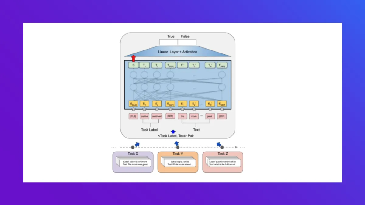
For text classification, zero shot learning can be done by exploiting natural language Inference (NLI) models. In NLI, you have a premise and a hypothesis. The model has to predict the relationship between the two sentences:
- Entailment (the premise implies the hypothesis)
- Neutral (no obvious relationship)
- Contradiction (the premise contradicts the hypothesis)
To perform zero shot text classification, you consider the document you want to classify as the premise. The hypothesis then becomes a sentence of the form: "This document is about LABEL". Then you make predictions using a BERT model for each of the labels that you have. To get a text classification output, take the probability given by the model for entailment. The label that has the highest probability can be interpreted as being the one that is most likely.
That's it! You have done text classification without training a model and without gathering any training data.
What you need to know
The quality of the results you’ll get depends strongly on the semantics of your labels. Labels that are actual words will work better than abbreviations or codes, so with “Shovels” BERT will have something to compare against, unlike CPC code “A01B1/02”.
Another thing that can influence the results is the template used for the hypothesis. The generic template (“This document is about LABEL”) should be replaced with something more specific, depending on the use case.
Pros and cons of this approach
A big advantage of ZSL is that you only need 5 lines of code in a Jupyter Notebook to get started. It will take you longer to come up with the relevant labels for your dataset than it does to get the whole thing running. Another advantage of ZSL is that you can add new labels, or even new tasks, without having to retrain a model.
The downside is that this approach doesn’t have the highest accuracy. For example, on the Yahoo Answers dataset, which has 10 classes, you can get around 50% accuracy using a BART-large model for the NLI problem.
Another drawback of ZSL is that you have to run inference once for every label, so if you have many labels, this can be inefficient. The good news is that distillation (which we’ll discuss below) is a solution for that.
Overall, zero shot learning is a game changer for creating quick demos and proof of concepts, which are needed to get buy-in from the customer who is skeptical about machine learning.
Few-Shot Learning
What is it?
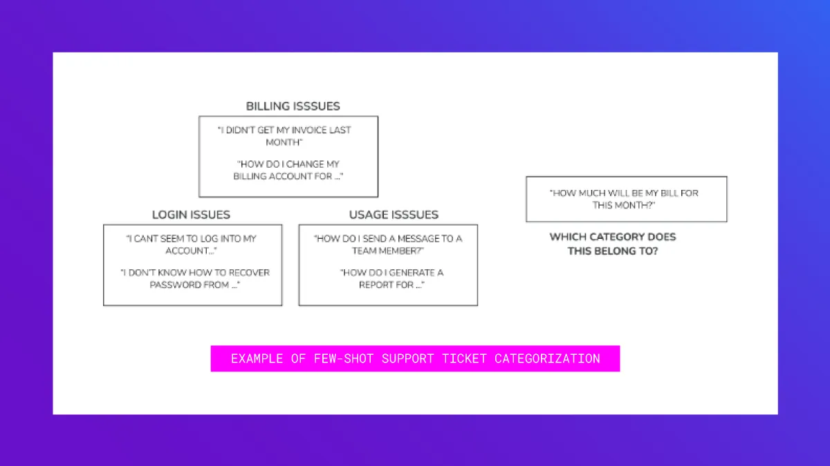
Few-shot learning (FSL) – sometimes referred to as low-shot learning – is a more generalized version of zero-shot learning. In this case, the “few shots” refer to the examples you have for each of your target classes.
Whereas traditional machine learning techniques try to fit a model to large data sets where each class may have thousands of examples, an FSL model is trained on limited data. For example, each class may have only a handful of examples.
How it works
Typically, if there are k classes and n examples in each class, we refer to the learning task as k-way n-shot learning.
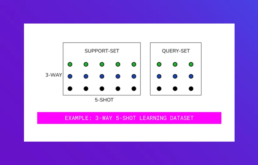
In FSL, the model learns to learn how to discriminate between examples in one class versus the other. This helps the model work well, even on an unseen task – i.e. where the model has never seen the classes or the examples you want to classify on. In that sense, it is a form of meta-learning. Here’s what you need to know to get started.
What you need to know
At training time, you have a few examples in each of your classes. Since we want to train the model on how to distinguish between examples in one class versus another, we train the model as multiple “tasks” that teach the model how to discriminate. In each task, you take a subset of k classes. Additionally, you split the n examples you have into your support set and query set.
Each task is thus structured similar to a k-way n-shot task (albeit, with a subset of k classes and n examples). Each step in this learning optimizes for the loss (or error) on the query set. By repeatedly learning on such randomly selected subsets of k and n, the model learns to discriminate between unseen examples.
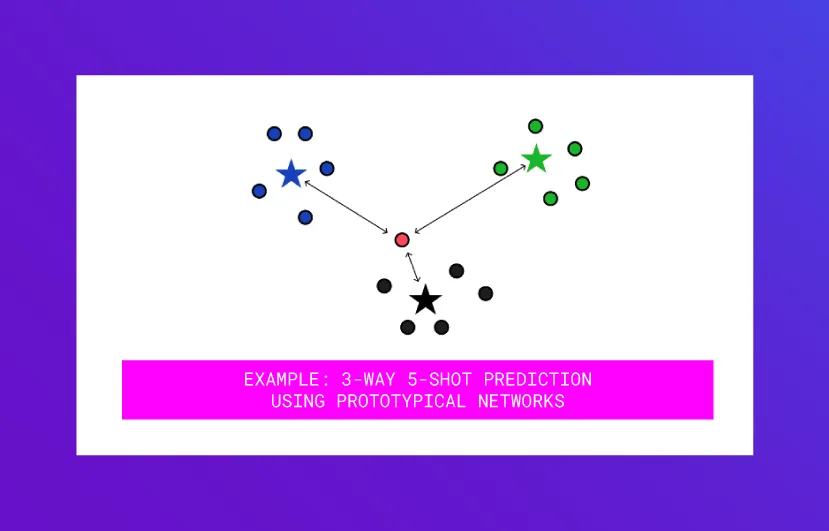
At testing time, you may present the model with k classes that were never part of the training tasks, and n examples that the model has never seen. For example, in prototypical networks (a method we dig a little deeper into later) the embedding of the example to be predicted is compared to the means of the embeddings of the new n examples in the k unseen classes to predict its class membership.
Typical methods for few-shot learning are Matching Networks, Prototypical Networks, Graph Networks, Induction Networks, etc. and are compared in this paper where model performance is evaluated on 1-shot, 5-shot, or 10-shot tasks on systematic subsets of the data. This recent paper lists benchmarks that are actively being researched - for example Open Domain Intent Classification for Dialog System (or ODIC) dataset and Real-World Few-Shot Text Classification Benchmark (or RAFT).
Pros and cons of this approach
One benefit to this approach is that it relies on few examples of labeled data. It’s also easy to implement and you can expect quick results.
In terms of disadvantages, learning the embedding function can still take some time. It’s also still in the early stages. Text and image categorization are well researched, but other few-shot tasks (e.g. NLP, segmentation) are not yet well researched. Finally, it does not use the label semantics lik zero-shot learning.
Use case
Prototypical Networks are a great starting point to working with few-shot learning because the method is simple, and easy to implement.
Here’s the general idea: For each example in our training set, we generate an embedding. We then create a “prototype” of a class by averaging the embedding for all examples in that class.
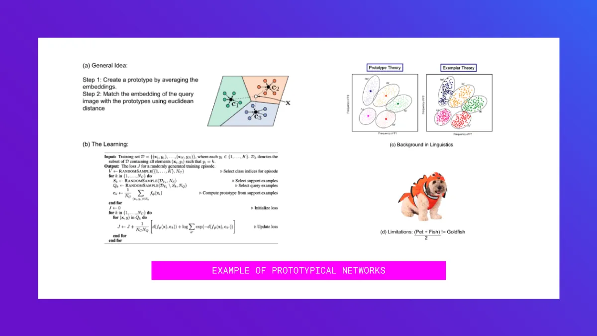
During prediction time, for a text we want to classify, we calculate euclidean distances of that data point from all the prototypical centroids, and then take a soft-max of those distances to calculate prediction probabilities of class memberships. (See a in the image above)
Since the prediction methodology is pretty simple, one could say that the “magic” lies in generating the right embeddings. The original paper on Prototypical Networks that learned the embedding space uses the hold-out approach described earlier. In each training task, they took a subset of the k classes to learn and split the n examples into a support and query set. The neural network learned using the loss on the query set. The embeddings generated were thus able to discriminate between the classes. (See b in the image above). Check out the code for the Prototypical Networks paper and also a more detailed explanation and example of the approach in this article.
A lot has been written on prototype theory in linguistics, which is often contrasted with exemplar theory. In machine learning, the analogy for the prototype theory is k-means and that for exemplar theory is n-nearest neighbors (See c in the image above). Likewise, a lot of literature covers the limitations of prototype theory. Some classes cannot be constructed with the mean method. For example the mean of pets and fish is not going to be a gold-fish (See d in the image above). You can read more on prototype theory here.
Weakly supervised learning
What is it?
If you have a large unlabeled data set and are able to describe your mental classification process with rules and heuristics, weakly supervised learning together with data programming might come handy.
How it works
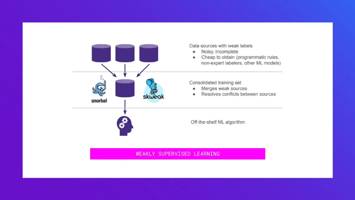
With weakly supervised learning, you code each rule and heuristic as a programmatic function – also called a labeling function – that maps each of your unlabeled data points either to a class label or abstains. Importantly, these labeling functions need not be a hundred percent accurate. Being sufficiently better than random is enough.
A weakly supervised learning algorithm such as Snorkel or those implemented in skweak then combines the votes of the individual labeling functions, resolves conflicts, and outputs a training dataset with probabilistic labels that you can then plug into off-the-shelf classification models.
What you need to know
While you can use existing dictionaries and ontologies to bootstrap your rule set, in order to refine the rule set, a data scientist together with a subject matter expert can go through an iterative process where they:
- Discover new rules through inspecting the resulting classification output or looking at data points which are not yet covered by any rule.
- Tune and test the rule through manual inspection or on a small validation set
- Add the rule to your rule set
Frameworks such as Rubrix facilitate this kind of explorative analysis.
Pros and cons of this approach
Weakly supervised learning through data programming has the following advantages over classical manual annotations:
- Rules contain more information while still being quick to formulate
- Subject matter experts are forced to explicitly formulate their rational
- A set of rules is easier to review and govern, e.g. when facing concept drift
However, there are a few constraints when applying data programming:
- It works best on classification problems with text and tabular data.
- Even for some classification problems it’s hard to come up with sensible rules (e.g. sentiment analysis)
- Labeling functions ideally find a sweet spot between being highly accurate but covering only a few examples vs. being noisy but broad.
Use case
One good example for weakly supervised learning is document retrieval when it is too complex to express the rational of what a relevant or irrelevant document is as a search query of existing frameworks (e.g. ElasticSearch). Instead, users can formulate heuristics of what makes a document relevant or irrelevant. A data programming workflow in this setting could comprise of:
- Bootstrapping a rule set by transforming keywords into rules for the relevant class
- Refining the rule set in an interactive session between a data scientist and the expert user
In less than an hour, you’ve configured a custom tailored document retrieval system. The user is put into the driver seat: by defining rules she can directly shape what the retrieval system is doing.
Zero–label models
What is it?
Zero-label learning is a new approach to leverage large language models (LLM), such as GPT-3, to learn from unlabeled data. You can read the full Google research paper, Wang et al., Towards Zero-Label Language Learning, arXiv 2021.
How it works
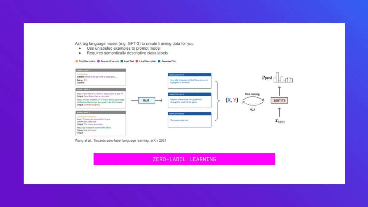
The main idea is unsupervised data generation. First, you engineer a prompt that consists of:
- Some unlabeled examples to familiarize the LLM with what typical examples in your dataset look like
- An instruction to generate a new example for a certain class (i.e. 3/5 star review on Yelp)
The LLM will then generate a new data point based on the prompt. Repeat this process until a suitably large training data set is generated. From that training set, you can then train a downstream machine learning model. The resulting accuracy is on-par with few-shot methods that require a few labeled examples. The method can also be used to augment labeled data sets.
Overall, this paper provides a tool that’s handy for certain problem sets and it demonstrates once again the generative versatility of large language models.
What you need to know
Since the generated training examples might be of low quality, the paper proposes using a noise-aware downstream model that allows you to filter low-quality training samples.
The paper not only uses this approach to learn with zero true labels. Additionally, they look at complementing a small labeled data set with artificially created training samples, allowing you to achieve superhuman performance on the SuperGLUE benchmark.
Pros and cons of this approach
Zero-label learning allows you to distill the vast amount of knowledge embedded into foundational large language models. This comes with a number of advantages. First, zero-label learning doesn’t need any labeled data. Second, the LLM needs to be queried only to generate training data. After deployment, the downstream classifier will predict on new data. Hence, the inference costs of the LLM amortize over time.
However, there are some disadvantages to this approach. First, your target concepts need to be expressible in natural language and you need to engineer suitable task descriptions. You also need to deal with low quality samples, either through manual review or by using a noise-aware downstream classifier.
Use case
The paper demonstrates the effectiveness of zero-label learning on various tasks, from the classification of product reviews and tasks that require the disambiguation of the meaning of single words in sentence, all the way up to high-level common-sense reasoning tasks.
On the SuperGLUE benchmark, the paper shows that zero-label learning is on-par with few-shot learning despite not having access to any label. Also on SuperGLUE, the paper shows that unsupervised data generation can enrich labeled training data sets. For the first time, they achieve a level of accuracy that surpasses an estimated human baseline.
Distillation/teach-student models
What is it?
Often, even if you get good results with a large model, you might want to use a smaller model for faster inference or because it’s less resource intensive. You can do this using distillation by having the large model (teacher) give extra knowledge to the small model (student).
How it works
Distillation works by generating a pseudo labeled dataset using the teacher model and then having the smaller model learn on that dataset.
One way to do this is to take a small amount of labeled data and a large amount of unlabeled data. The teacher model is trained on the labeled data and it then classifies the unlabeled data. The resulting predictions will form the pseudo-labeled dataset on which the student model is trained.
This can also be used in the case of zero shot models, if you have access to some unlabeled data. You use the ZSL models to classify that unlabeled data and then you can train a regular model on that data.
What you need to know
Distillation enables smaller models to reach performances that they couldn’t reach by training on their own on the normal dataset. By having access to a larger model, which has more capacity, the small model can learn the most relevant features directly.
Pros and cons
The advantage of distilling zero shot models to a regular model is that inference becomes more efficient because you don't have to run the model once for each class. When distilling normal models, the advantage is that you get a smaller model that can run faster, with less resource usage.
While distillation can be used to obtain a much more efficient model, the disadvantage is that the whole training pipeline becomes more complicated and you have to keep track of two models.
Use case
To give a brief example from work we did: on one text classification project with about 30 classes with about 1000 labeled documents, a simple Logistic Regression model gave about 60% accuracy. A BERT large model trained on the same data reached 75% accuracy. Because we had access to about 30000 more unlabeled documents, we could predict the labels for those documents using the BERT large model and were able to retrain the Logistic Regression on this extended dataset. The results were quite good: now the Logistic Regression gave about 70% accuracy.
From weeks to hours
Modern NLP models such as BERT and GPT-3 are really powerful and contain enough knowledge to perform many tasks with very little fine tuning. When you combine these with techniques like model distillation and weakly supervised learning, you can get started with new NLP projects and show results in hours instead of weeks.
This article was a recap of a Tribe AI event, "No labels are all you need – why your labels suck and what you can do about it." To learn more about training with little to no data, reach out to the authors Rahul Parundekar, Roland Szabo, and Tobias Plötz. Want to join our next event? Apply to join our collective of 200+ ML engineers and data scientists.


